Defining models

This section explains how to define models through python calls.

Defining cluster models

Clusters are the building blocks of lattice models. One needs to define them first. This is done through calls to new_cluster_model(). For instance:

from pyqcm import *
new_cluster_model('2x2_C2v', 4, 0, [[3, 4, 1, 2], [2, 1, 4, 3]])

The function new_cluster_model(name, Ns, Nb, perm, bath_irrep) takes the following arguments:

1. A name given to the cluster model

2. The number \(N_s\) of physical sites

3. The number \(N_b\) of bath sites

4. (optional) A list of permutations of the \(N_o=N_s+N_b\) orbitals that define generators of the symmetries of the cluster.

5. (optional) A boolean flag that, if true, signals that bath orbitals belong to irreducible representations of the symmetry group of the cluster, instead of being part of permutations of the different orbitals of the cluster-bath system.

In the above example, a four-site cluster is defined, without any bath sites. The positions of the sites are not relevant to the impurity solver, and so are not defined at this stage. However, a plaquette geometry is implicit here, with the following site labels:

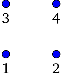
Figure 1

The cluster symmetries (permutations) passed to the function thus correspond to reflexions with respect to the horizontal and vertical axes, respectively. The cluster symmetries will be used by the ED solver to lighten the exact diagonalization task. Large clusters will take less memory, convergence of the Lanczos method will be faster, and computing the Green function at a given frequency will be more efficient. The different permutations that constitute the generators must commute with each other. They generate an Abelian group with \(g\) elements. Such a group has an equal number \(g\) of irreducible representations, numbered from 0 to \(g-1\).

Defining operators on the cluster

Most operators in the model are best defined on the lattice and their restriction to the cluster is defined automatically, so there is no need to define them explicitly on each cluster of the super unit cell. This is not the case if one wants to use the ED solver as a standalone program without reference to a lattice model. Bath operators, on the other hand, need to be defined explicitly within the cluster model since they do not exist on the lattice model.

The following code defines the cluster and bath operators for the cluster illustrated in the last section, which we reproduce here:

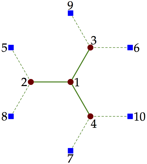
Figure 2

Content of the cluster definition file:

from pyqcm import *

no = 10
ns = 4
new_cluster_model('clus', ns, no-ns, [[1, 3, 4, 2, 6, 7, 5, 9, 10, 8]])


new_cluster_operator('clus', 'bt1', 'one-body', [
    (2, 5, 1.0),
    (3, 6, 1.0),
    (4, 7, 1.0),
    (2+no, 5+no, 1.0),
    (3+no, 6+no, 1.0),
    (4+no, 7+no, 1.0)
])

new_cluster_operator('clus', 'bt2', 'one-body', [
    (2, 8, 1.0),
    (3, 9, 1.0),
    (4, 10, 1.0),
    (2+no, 8+no, 1.0),
    (3+no, 9+no, 1.0),
    (4+no, 10+no, 1.0)
])

new_cluster_operator('clus', 'be1', 'one-body', [
    (5, 5, 1.0),
    (6, 6, 1.0),
    (7, 7, 1.0),
    (5+no, 5+no, 1.0),
    (6+no, 6+no, 1.0),
    (7+no, 7+no, 1.0)
])

new_cluster_operator('clus', 'be2', 'one-body', [
    (8, 8, 1.0),
    (9, 9, 1.0),
    (10, 10, 1.0),
    (8+no, 8+no, 1.0),
    (9+no, 9+no, 1.0),
    (10+no, 10+no, 1.0)
])

Note that the symmetry defined here is a rotation by 120 degrees. This generates the group \(C_3\), which has complex representations. pyqcm can only deal with Abelian groups (the correct treatment of non-Abelian symmetries is too complex when computing Green functions for the benefits it would provide). In the above example, a better strategy when no complex operators are present would be to define only a \(C_2\) symmetry based on one of three possible reflections. This would only provide 2 symmetry operations instead of 3, but the representations would be real instead of complex, thus saving more time and memory.

The function new_cluster_operator(model, name, type, elements) takes the following arguments:

1. The name of the model (the same given to new_model())

2. The name of the operator

3. The type of operator; one of ‘one-body’, ‘anomalous’, ‘interaction’, ‘Hund’, ‘Heisenberg’

4. An array of real matrix elements. Each element of the array is a 3-tuple giving the labels of the orbitals involved and the value of the matrix element itself. Note that spin-up and spin-down orbital labels are separated by the total number of orbitals on the custer, here no=10.

If a complex-valued operator is needed, then the function new_cluster_operator_complex() must be used, the only difference being that the actual matrix elements are complex numbers.

Defining lattice models

A simple example

The following simple example illustrates how to define a Hubbard model on the square lattice in two dimensions:

from pyqcm import *

new_cluster_model(clus', 4, 0, [[4, 3, 2, 1]])
add_cluster('clus', [0, 0, 0], [[0, 0, 0], [1, 0, 0], [0, 1, 0], [1, 1, 0]])
lattice_model('2x2_C2', [[2, 0, 0], [0, 2, 0]])
interaction_operator('U')
hopping_operator('t', [1, 0, 0], -1)
hopping_operator('t', [0, 1, 0], -1)
hopping_operator('t2', [1, 1, 0], -1)
hopping_operator('t2', [-1, 1, 0], -1)
hopping_operator('t3', [2, 0, 0], -1)
hopping_operator('t3', [0, 2, 0], -1)
anomalous_operator('D', [1, 0, 0], 1)
anomalous_operator('D', [0, 1, 0], -1)
density_wave('M', 'Z', [1, 1, 0])

There is a call to new_cluster_model() to define a \(2\times2\) plaquette with a \(C_2\) symmetry (rotation by 180 degrees). Then this cluster is added to the lattice model via the function add_cluster() which takes 3 arguments:

1. The name of the cluster model (here clus)

2. The base position of the cluster within the super unit cell (here [0,0,0])

3. An array of integer positions of the different cluster sites. This is where the geometry of the cluster appears.

The funcion add_cluster() is used to add individual clusters to the super unit cell. Only at the end of this process can the lattice model itself be defined properly by the function lattice_model(), which is the signal that no more clusters are needed. In the above example, the super unit cell contains a single cluster. Therefore add_cluster() is called only once and the lattice model can then be wrapped up by a call to lattice_model(), which takes three arguments (the last one optional):

1. The name of the model, for reporting purposes

2. The \(d\) vectors defining the superlattice vectors. \(d\) is the dimension of the model.

3. The \(d\) vectors defining the lattice vectors of the model. In the above example this is omitted because the default value is used: [[1,0,0], [0,1,0]].

Note that all vectors used in these specifications have three components (even for lower dimensional models) and have integer components. They are in fact coefficients of basis vectors generating a working Bravais lattice and are therefore integers by definition (not all vectors of this working Bravais lattice need belong to the actual Bravais lattice of the model; the case of the graphene lattice is illustrated below).

Once the geometry of the model is defined, operators can be added to the model via various functions. The Hubbard on-site interaction is added with a call to interaction_operator('U'), whose sole argument in this case is the name we choose for that operator (more arguments are needed for other types of interactions, multi-band models, etc; see the detailed documents in the reference section on functions).

Nearest-neighbor hopping is defined with a call to hopping_operator(), which has three mandatory arguments:

1. The name of the operator

2. The link on which the operator is defined

3. The amplitude of the operator on that link.

Optional keyword arguments are needed for multi-band models, spin-flip operators, etc. In the above example this function is called twice with the same name but different links (along [1,0,0] and [0,1,0] respectively). The matrix elements generated by the two calls are simply added to the list associated with this operator. Similar calls are performed for the second-neighbor hopping t2 and the third-neighbor hopping t3.

A d-wave pairing operator is defined via a call to anomalous_operator() , which takes the same arguments as hopping_operator(), i.e., name, link and amplitude. Note that two calls are made with the same name D, one in the \(x\) direction, the other one in the \(y\) direction, with amplitudes 1 and -1, in accordance with the d-wave character of the operator.

Finally, a density wave corresponding to \((\pi,\pi)\) antiferromagnetism is added, with a call to density_wave(), which has 3 mandatory arguments:

1. The name of the operator (here ‘M’)

2. The type of density-wave (here ‘Z’ for a spin density wave in the \(z\) component of the spin). Other possibilities are:

   • ‘N’ : charge density wave

   • ‘X’ : spin density wave in the \(x\) component of the spin

   • ‘spin’ : same as Z

   • ‘singlet’ : singlet pairing

   • ‘dx’ : triplet pairing in the \(x\) direction using the \(\mathbf{d}\) vector formalism.

   • ‘dy’ : same, in the \(y\) direction

   • ‘dz’ : same, in the \(z\) direction (this one does not require Nambu doubling)

3. The wavevector \(\mathbf{Q}\) of the density wave. It has real components (in multiples of \(\pi\)) and it must be commensurate with the super unit cell within some small numerical tolerance.

Additional keyword arguments to density_wave() include the link on which the density wave is defined (for bond-density waves), lattice orbitals involved (for multi-band models), additional phases and amplitudes, etc. Again, see the reference section for details.

A more complex example

The following example defines a model on the graphene lattice using two cluster within the super unit cell and the graphene lattice, as illustrated below:

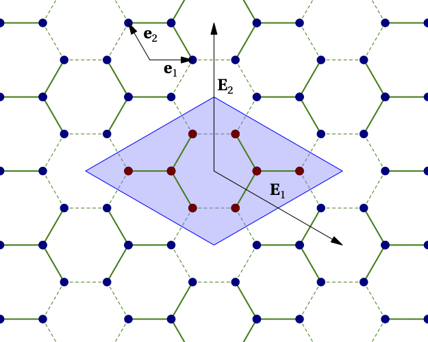
Figure 3

Of possible set of function calls to define the Hubbard model on this system is:

import cluster_h4_6b_C3
from pyqcm import *

add_cluster('clus', [-1, 0, 0], [[0, 0, 0], [-1, 0, 0], [1, 1, 0], [0, -1, 0]])
add_cluster('clus', [1, 0, 0], [[0, 0, 0], [1, 0, 0], [-1, -1, 0], [0, 1, 0]])
lattice_model('h4_6b_C3', [[2, -2, 0],[2, 4, 0]], [[1, -1, 0], [2, 1, 0]])
set_basis([[1, 0, 0], [-0.5, 0.866025403784438, 0], [0, 0, 1]])

interaction_operator('U')
hopping_operator('t', [1,0,0], -1, orbitals=(2,1))
hopping_operator('t', [0,1,0], -1, orbitals=(2,1))
hopping_operator('t', [-1,-1,0], -1, orbitals=(2,1))

The first statement, import cluster_h4_6b_C3, imports a cluster definition file, for instance the one associated with Fig. 2 above. Using the name clus given to the cluster in that file, two copies of the clusters are added to the super unit cell. The positions associated with the two copies are different, but the cluster model is the same, which means that only one copy of the Hilbert space operators and bases necessary for the exact diagonalization will be constructed. The origin has been placed exactly between the two clusters. The positions in each cluster are defined relative to the base position of each cluster.

The integer positions are defined in terms of the basis defined by the call to set_basis(). The argument of that function is a set of real-valued vectors defining the basis vectors of the working Bravais lattice. On Fig. 3, the first two of these vectors are \(\mathbf{e}_1\) and \(\mathbf{e}_2\).

The call to lattice_model() defines both the superlattice vectors \(\mathbf{E}_1\) and \(\mathbf{E}_2\) (second argument) and the basis vectors of the model’s physical Bravais lattice (third argument). The lattice basis vectors only serve to attribute orbital labels to the different sites. In qcm, each degree of freedom of a given spin (i.e. each orbital) must have its own site on the working Bravais lattice. The basis vectors of the physical Bravais lattice then define orbital labels (from 1 to \(N_\mathrm{band}\)) attributed to each site. The order in which orbitals are labelled depends on the order in which the sites appear. Given the above definitions and Fig. 3, the A sublattice of graphene corresponds to orbital 2 and the B sublattice to orbital 1.

Given that the model has two bands, the definition of the hopping operator t must contain orbital information: the keywords orbitals (a tuple) is used to specify the orbital numbers associated with the two sites separated by the bond vector (link) given in argument. Internally, a loop is done over all sites of the super unit cell; the bond vector is used to identify a second site; if that site exists and if the orbitals associated with the two sites agree with orbitals, then a matrix element is added to the operator. In the above example, three calls are needed because of the three directions (bonds).

The greatest risk in such calls is to mislabel the orbitals. In order to check that operators were defined properly, a call to print_model() is warranted. This function takes one mandatory argument: the name of a text file in which a detailed enumeration of model properties will be printed. Additional keyword arguments control the production of asymptote files (.asy) that graphically illustrate each operator. This is a powerful way to check the validity of the model definition.

Other examples

The distribution contains a folder (notebooks) that contains many examples of models and codes. New users are encouraged to study a few of these models and to consult the reference section for more detailed information about model building.