Models and clusters
Pyqcm can be applied to Hubbard and extended Hubbard models with one or more bands defined in 0 to 3 dimensions of space. These models are defined on a lattice, which may not be a Bravais lattice, but which contains a Bravais lattice as a subset. In other words, the sites of the lattice constitute the Bravais lattice itself and its basis within each unit cell.
Lattices and superlattices
In quantum cluster methods, the lattice is divided into repeated units that are generally (but not necessarily) larger than the unit cell. The repeated unit is called the the super unit cell (SUC) and is made of one or more clusters. The repetition defines a superlattice. For instance, the figure below shows how the honeycomb lattice is tiled with an 8-site super unit cell (shaded in blue), itself made of two 4-site clusters. The original Bravais basis vectors are \(\mathbf{e}_1\) and \(\mathbf{e}_2\). The superlattice vectors are \(\mathbf{E}_1\) and \(\mathbf{E}_2\). The inter-cluster links are indicated by dashed lines and the intra-cluster links by full lines.
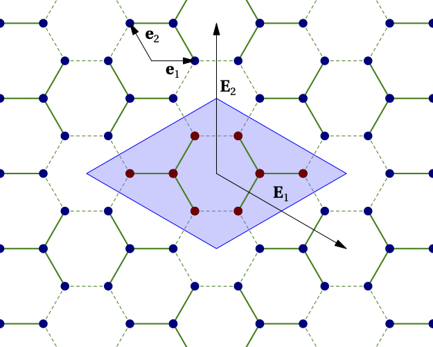
Figure 1
Another example is the triangular lattice, where the supercell can be made of a two contiguous and inverted 15-site triangles, each of them being a cluster with the point group of the lattice, but not a repeatable pattern on the lattice. Only by adjoining two such clusters does one recover a repeatable unit:
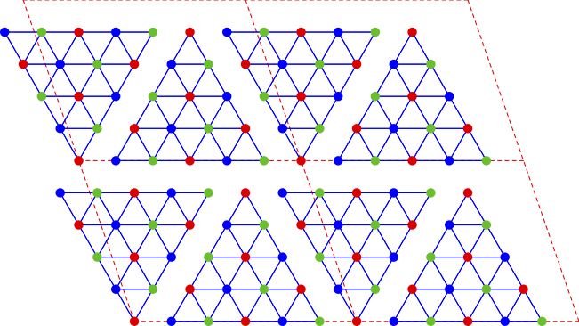
Figure 2
Note that the triangular lattice is often thought of as made of three intertwined sublattices (A, B and C) whose sites are represented in blue, red and green on the figure. Note that the 15-site cluster treats these three sublattices symmetrically, which is useful when studying spiral magnetic order based on these three sublattices.
Let us summarize:
A model is defined on a lattice of dimension \(D\)
Cluster methods assume that this lattice is an assembly of small clusters and that a small number (possibly one) of these clusters form a repeated unit forming the basis of a superlattice of dimension \(D\)
Lattice models
In quantum cluster methods, one deals with a Hubbard-like model defined on the infinite lattice, the so-called lattice model, which we are attempting to solve approximately. The road to this approximate solution goes through defining closely related models on small clusters (the so-called impurity models), but more on this below. Let us start by explaining the range of lattice models that can be studied and defined in pyqcm.
Lattice models are defined by a Hamiltonian in dimension \(D=0,1,2\) or 3. \(D\) is the dimension of the Brillouin zone, i.e. the number of directions in which the model is infinite and a basic unit periodically repeated. For instance, one could consider a two-dimensional Hubbard model (a frequent case), or maybe a two-dimensional model with a finite number of layers in the third dimension, for instance to study heterostructures or a slab geometry, which still constitutes a two-dimensional model because it is infinite in two directions only. The model is made of one-body terms and interaction terms and has the general form
where each index \(a\) represent either a one-body operator or an interaction term, and \(h_a\) is the (real) value of the coefficient of each term. The operator \(H_a\) is Hermitian.
The parameters \(h_a\) of the lattice model are commonly referred to as ‘lattice parameters’ in this document and in the code, to distinguish them from the parameters of the various cluster Hamiltonians that make up the lattice.
In the code, the definition of an operator \(H_a\), the value of its coefficient \(h_a\) in the Hamiltonian and of its expectation value \(\langle H_a\rangle\) are encapsulated in the same data structure, so that the same symbol is often used to refer to all three concepts. This has to be kept in mind in this manual. When we say the value of operator \(H_a\), we mean the value of its coefficient \(h_a\), and we sometimes use the words operator and parameter interchangeably.
One distinguishes the following types of terms:
One-body operators
where each of the indices \(\alpha\) and \(\beta\) stands for a given site and spin (composite index \((i,\sigma)\)). The hopping amplitude matrix \(t^{(a)}_{\alpha\beta}\) is Hermitian. For a given pair of sites, labelled 1 and 2, the general form of the one-body term is
The use of Pauli matrices \(\sigma^b_{\alpha\beta}\) and \(\tau^a_{ij}\) makes sure that the operator is Hermitian (\(a=0\), \(b=0\) correspond to the identity matrix). Case \(a=1\) and \(b=0\) corresponds to an ordinary hopping term, without spin flip. In specifying the precise shape of the one-body operator, it will suffice to specify the matrix types \(a\) and \(b\) for the spatial and spin parts respectively.
Anomalous operators
Anomalous (or pairing) operators are useful in describing superconductivity. They have the general form
where again the indices \(\alpha\) and \(\beta\) are composite indices. The pairing amplitude \(\Delta^{(a)}_{\alpha\beta}\) is antisymmetric. It may be symmetric in site indices and antisymmetric in spin indices (singlet superconductivity), or vice-versa (triplet superconductivity). A common way of representing these possibilities is the so-called d-vector :
where the index \(b\) can take the values 0 to 3. The case \(b=0\) corresponds to singlet superconductivity (in which case \((\Delta^{(a)}_{ij,0} = \Delta^{(a)}_{ji,0}\)) and the cases \(b=1,2,3\) corresponds to triplet superconductivity (in which case \((\Delta^{(a)}_{ij,b} = -\Delta^{(a)}_{ji,b}\)).
pyqcm provides functions to define pairing operators by specifying the vectors \(i-j\) and the values of \(b\).
Density waves
Density wave operators are defined with a spatial modulation characterized by a wave vector \(\mathbf{Q}\). They can be based on sites or on bonds. If the operator is a site density wave, its expression is
\[x\sum_\mathbf{r} A_\mathbf{r} \cos(\mathbf{Q}\cdot\mathbf{r}+\phi)\]where
\[A_{\mathbf{r}} = n_{\mathbf{r}}, S^{z}_\mathbf{r}, S^{x}_\mathbf{r}\]If it is a bond density wave, its expression is
\[\sum_{\mathbf{r}} \left[ x c_\mathbf{r}^\dagger c_{\mathbf{r}+\mathbf{e}} e^{i(\mathbf{Q}\cdot\mathbf{r}+\phi)} + \mathrm{H.c} \right]\]where \(\mathbf{e}\) is the link vector.
If it is a pair density wave, its expression is
\[\sum_{\mathbf{r}} \left[ x c_\mathbf{r} c_{\mathbf{r}+\mathbf{e}} e^{i(\mathbf{Q}\cdot\mathbf{r}+\phi)} + \mathrm{H.c} \right]\]where \(\mathbf{e}\) is the link vector and \(\mathbf{r}\) a site of the lattice.
In pyqcm the different types of density waves are associated with keywords:
‘N’ : normal, i.e., a charge density wave
‘Z’ or ‘spin’ : a spin density wave, for \(S_z\)
‘X’ : spin density wave, for \(S_x\)
‘singlet’ : a pair-density wave, with singlet pairing. In this case and the following, the first creation operator in the above equation is replaced by an annihilation operator.
‘dx’, ‘dy’ ‘dz’ : a pair density wave, with triplet pairing, with d-vector in the directions x, y or z.
On-site interaction terms
Interaction terms can of the Hubbard or extended Hubbard type. The Hubbard on-site interaction is expressed as
where \(n_{is}=c^\dagger_{is} c_{is}\) is the number operator at site \(i\) and spin projection \(s=\uparrow,\downarrow\).
Extended interaction terms
The extended (Coulomb) interaction is expressed as
Hund’s coupling terms
It is also possible to add a Hund’s coupling term:
where \(i\) and \(j\) stand for site indices and where
See, e.g., A. Liebsch and T. A. Costi, The European Physical Journal B, Vol. 51, p. 523 (2006). This can also be written as
or as
Heisenberg coupling terms
Finally, it is possible to add a Heisenberg coupling term:
Clusters
A cluster is a unit of the system (or impurity, in the DMFT jargon) that is solved exactly by the impurity solver, in our case by exact diagonalization. There may be more than one cluster in the repeated unit (or super unit cell). The spatial correlations are exactly taken care of only within the cluster. The size of the cluster is limited by the capacity to perform exact diagonalizations. Clusters may also be attached to bath sites, which are not part of the lattice model per se but serve to simulate each cluster’s environment in cluster (or cellular) dynamical mean field theory (CDMFT). The cluster Hamiltonian \(H'\), or reference Hamiltonian, has the same form as the lattice Hamiltonian (except for the possible presence of a bath), but the values of its one-body terms, noted \(h'_a\), may differ. The interaction terms are the same on the cluster and on the lattice. The case of extended interactions requires a special treatment because of the bonds broken across cluster boundaries, which must be treated within the Hartree approximation.
Multiband models
Multiband models are treated in pyqcm in a seemingly restrictive fashion, which in fact poses no restriction at all. It is assumed that each geometric site on the lattice correspond to a single orbital (with two spins). Models with more than one band must necessarily be accounted for by assigning differents sites to each lattice orbital. The perfect example of this is the Hubbard model on the honeycomb (aka graphene) lattice. The lattice is not a Bravais lattice, since it contains one vacancy for every two occupied sites on an underlying triangular lattice. But there is no obligation in qcm for the lattice to be a Bravais lattice, i.e., for every site of the lattice to be occupied by an orbital (empty sites are allowed). The reason for doing things this way is that sometimes the two lattice orbitals are equivalent, like in graphene. For instance, one can then define a 6-site cluster centered on a vacancy (the vertices of a hexagon). See Fig. 3 below. This cluster, interesting to use because of its symmetry, is a repeatable unit of the honeycomb lattice, but does not contain three identical unit cells of graphene, and could not be used if lattice orbitals were treated only on a unit-cell basis. The concept of lattice orbitals in fact is only relevant to the lattice itself, not to the clusters, which ignore it.
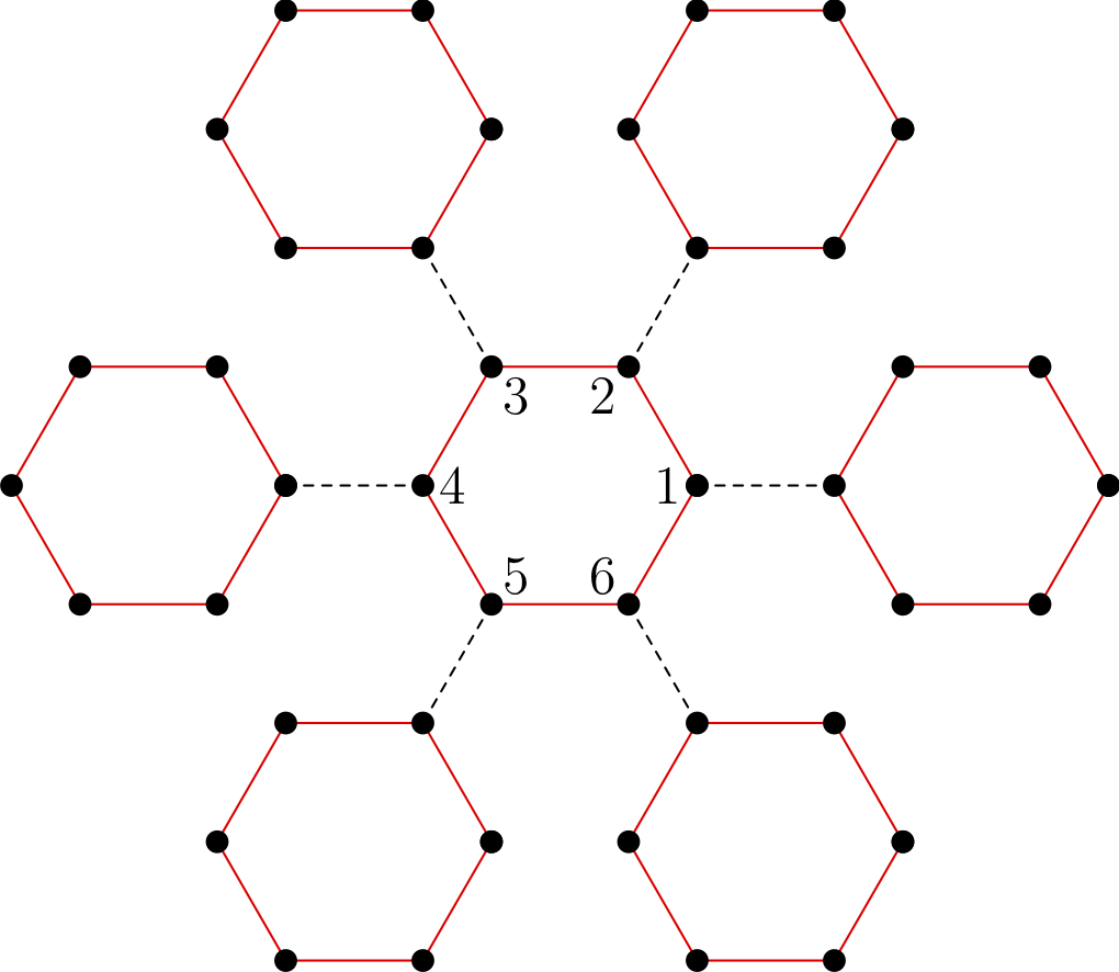
Figure 3
Bath sites
Each cluster can be associated with a bath of uncorrelated sites. This is illustrated on Fig. 4 for the four-site cluster of Fig. 1. From the point of view of the ED solver, the distinction between bath sites and physical sites is irrelevant. The only difference is that only physical sites have interactions. All the sites associated with a cluster are labelled consecutively, starting with the physical sites. The bath sites do not really have a position, even though they are pictured on Fig. 4 as if they occupied neighboring sites on the lattice.
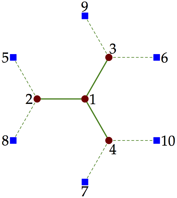
Figure 4
Site and orbital labels
By convention, orbitals (or degrees of freedom) within a cluster are numbered and labelled consecutively as follows, where \(N_s\) is the number of physical sites, \(N_b\) the number of bath sites, and \(N_o=N_s+N_b\):
From 0 to \(N_s-1\), the spin up orbitals of the cluster proper.
From \(N_s\) to \(N_o-1\), the spin up orbitals of the bath.
From \(N_o\) to \(N_o+N_s-1\), the spin down orbitals of the cluster proper.
From \(N_o+N_s\) to \(2N_o-1\), the spin down orbitals of the bath.
The above numbering is relevant to the ED solver but not to the lattice model. Instead, orbitals within the super unit cell are labelled in the order of consecutive clusters and keep the same ordering as they already have within clusters, except that bath sites are excluded. This means in particular that the spin down orbitals of the super unit cell are no longer grouped together; rather, it is the cluster index that is the most external index. Explicitly, the ordering of labels in the super unit cell is as follows:
From 0 to \(N_{s1}-1\), the spin up orbitals of cluster # 1 containing \(N_{s1}\) physical sites.
From \(N_{s1}\) to \(2N_{s1}-1\), the spin down orbitals of cluster # 1.
From \(2N_{s1}\) to \(2N_{s1}+N_{s2}-1\), the spin up orbitals of cluster # 2 containing \(N_{s2}\) physical sites.
From \(2N_{s1}+N_{s2}\) to \(2N_{s1}+2N_{s2}-1\), the spin down orbitals of cluster # 2.
etc.
Green function indices and mixing states
The above scheme describes the indices labeling the degrees of freedom. A slightly different scheme labels the indices of the Green function, depending on the mixing state:
Normal mixing. If there are no anomalous terms nor spin-flip terms in the model, then the Green function (cluster or lattice) does not mix up and down spins and the Gorkov function vanishes. The cluster Green function for cluster \(i\) is a \(N_{si}\times N_{si}\) matrix, associated with the destructions operators forming an array
The CPT Green function for the super unit cell (SUC) is then a \(N_s\times N_s\) matrix, where \(N_s\) is the total number of physical sites in the repeated unit:
This mixing state is called normal mixing.
Spin asymmetric mixing. If the model is not spin symmetric, i.e., if the up and down spins are not equivalent, then the down part of the Green function is different, but is still a \(N_s\times N_s\) matrix. This case is called spin asymmetric mixing. It entails separate computations for the up and down spin Green functions.
Spin-flip mixing. If there are spin-flip terms, but sill no anomalous terms, the cluster Green function is a \(2N_{si}\times 2N_{si}\) matrix, associated with the destructions operators forming an array
The CPT Green function for the SUC is then a \(2N_s\times 2N_s\) matrix, and the cluster index is the outermost index. This is called spin-flip mixing.
Simple Nambu mixing. If there are anomalous terms, but no spin-flip terms, the cluster Green function is a \(2N_{si}\times 2N_{si}\) matrix, associated with the destruction and creation operators forming an array
The CPT Green function for the SUC is then a \(2N_s\times 2N_s\) matrix, and the cluster index is still the outermost index. This is called simple Nambu mixing.
Full Nambu mixing. If there are both anomalous and spin-flip terms, the cluster Green function is a \(4N_{si}\times 4N_{si}\) matrix, associated with the destruction and creation operators forming an array
The CPT Green function for the SUC is then a \(4N_s\times 4N_s\) matrix, and the cluster index is still the outermost index. This is called full Nambu mixing. This also applies if there are no spin-flip terms, but triplet anomalous terms of the types dx`and `dy.
Different clusters may have different mixings, for instance if one of them describes a normal layer and another one a superconducting layer. However, the lattice model will have the more general mixing of the two and the Green function of each cluster will be upgraded to the lattice mixing as needed, for instance by doubling it by adding a Nambu transformed part.